Motivation
Random Forest 가 병렬적으로 무지 많은 Decision Tree를 만든다면, 부스팅에서는 Decision Tree를 점진적으로 발전시킨 후 이를 통합하는 과정을 한다.
AdaBoost와 같이, 중요한 데이터에 대해 weight를 주는방식 vs GBDT와 같이 딮러닝의 loss function 마냥 정답지와 오답지간의 차이를 다음번 훈련에 다시 투입시켜서 gradient를 적극적으로 활용, 모델을 개선하는 방식이 있는데, XGBoost, LightGBM이 이에(후자) 속한다.

LightGBM에서 (GOSS와 EFB방식을 통해) 번들을 구성, 데이터 feature를 줄여서 학습한다

Conventional GBM need to, for every feature, scam all data instances to estimate the information gain of all the possible split points.

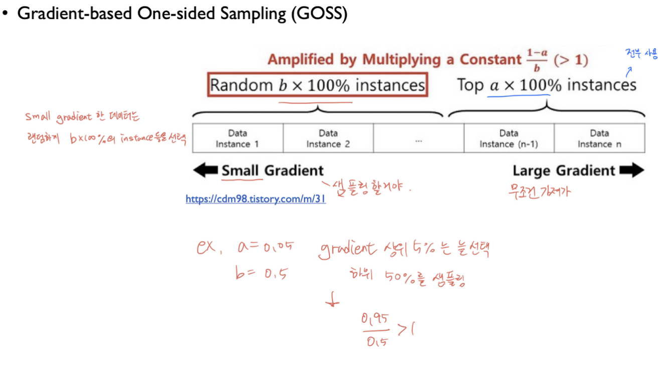
GOSS (Gradient-based One-Side Sampling)

1. Data instances with different gradients play different roles in the computation of information gain
2. Keep instances with large gradients and randomly drop instances with small gradients

1. 각 데이터들은 서로다른 gradient를 가지며, 이에대한 information gain이 다르다 -> 어느지점을 습득하는지에 따라 다른 역할을 수행하게된다.
2. large gradient한 데이터(instances)는 갖고가고, small gradient한 데이터에서 랜덤선택한다. -> 상위몇개를 고정, 하위몇개 중 랜덤하게 골라서 학습한다.

GBDT에서 모든 feature에 대해 스캔을 쭉 해서 가능한 split point를 찾아, information gain을 측정하는데, LightGBM에서는 모든 feature를 스캔하지않기위해, gradient-based One-Side Sampling 를 한다. (GOSS)

GBDT에는 weight는 없지만, gradient가 있다. 따라서 데이터의 개수를 내부적으로 줄여서 계산할 때, 큰 gradient를 가진 데이터는 그대로 사용하고, 낮은 gradient를 랜덤하게 drop하고 데이터를 가져와서, 샘플링을 해준다. gradient가 적다고 버리면 데이터 분포 자체가 왜곡될 수 있기에, 이대로 훈련하면 정확도가 낮아진다.

이를 방지하기위해 가져온 낮은 gradient 데이터에 대하여 ${1-a}\over{b}$ 만큼 뻥튀기 해준다.
(a: 큰 gradient데이터 비율, b: 작은 gradient 데이터 비율)

낮은 gradient를 가진 데이터만 drop하므로, One-Side Sampling이라고한다.
이렇게 feature를 줄여서 학습하는 것이다.

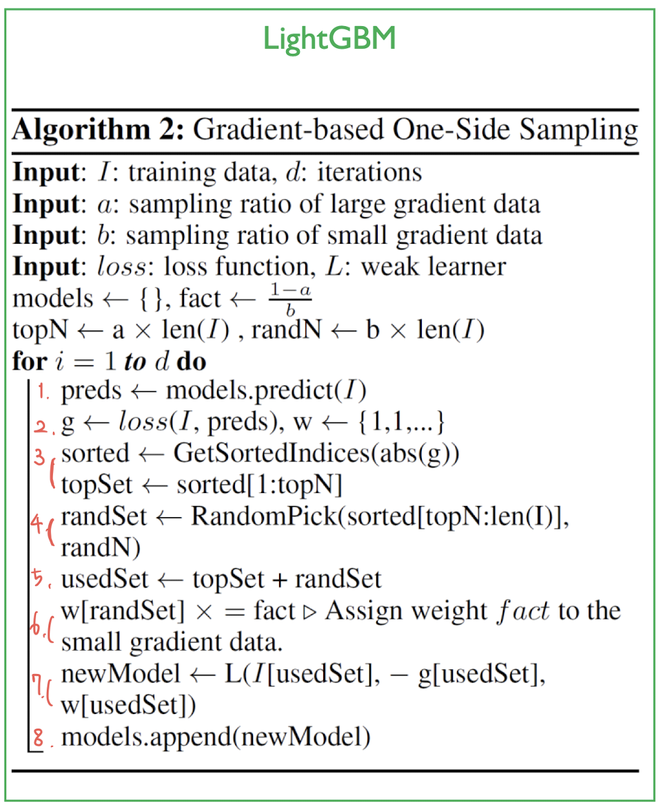
topN = a * len(I) ,전체 데이터의 a만큼 index (ex. 100개 중 a=0.2라면 topN=20)
randN = b* len(I) ,topN과 비슷하게 b만큼 index

1. 모델로 일단 예측
2. 실제값과의 error로 loss를 계산, weight를 계산하여 저장
3. loss대로 정렬 -> sorted에 저장. sorted[1:topN] 만큼 Loss 상위 데이터들 topSet에 저장 (ex. 전체 100개 중 a=0.2라면 20개)
4. 나머지 80개 중 randN개 만큼 랜덤샘플링하여 randSet에 저장 (ex. 나머지 80개 중 b=0.2라면 16개 데이터)
5. UsedSet에 topSet과 randSet을 저장
6. small gradient data에 fact(=${1-a}\over {b}$)만큼 weight를 부여해줌
7. weak learner를 만들어서 새로운 모델로 부여 , weak leaner에는 샘플링된 데이터(UsedSet = topSet + fact assigned randSet)와 loss와 weight가 들어감
8. 모델 저장

EFB (Exclusive Feature Bundling)

1. In a sparse feature space, many features are (almost) exclusive, i,e., they rarely take nonzero values simultaneously (ex. one-hot encoding)
2. Bundling these exclusive features does not degenerate the performance

1. 하나의 객체(feature)에 대해 특정 두개의 변수가 Non-Zero값을 갖는 경우가 드물다.
2. 그리하여 exclusive한 변수들을 번들링해도 성능저하가 거의 없다.

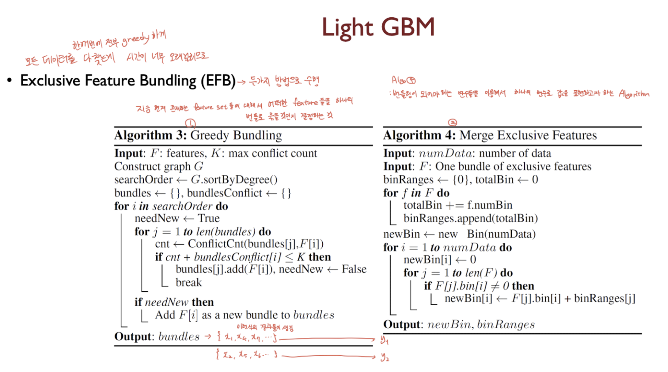
Greedy Bundling에서는 지금 현재 존재하는 feature set들에 대해서 어떠한 feature들을 하나의 번들로 묶을지 결정

Merge Exclusive Features에서는 번들링되어야하는 변수들을 이용, 하나의 변수로 값을 표현(Merge해줌)

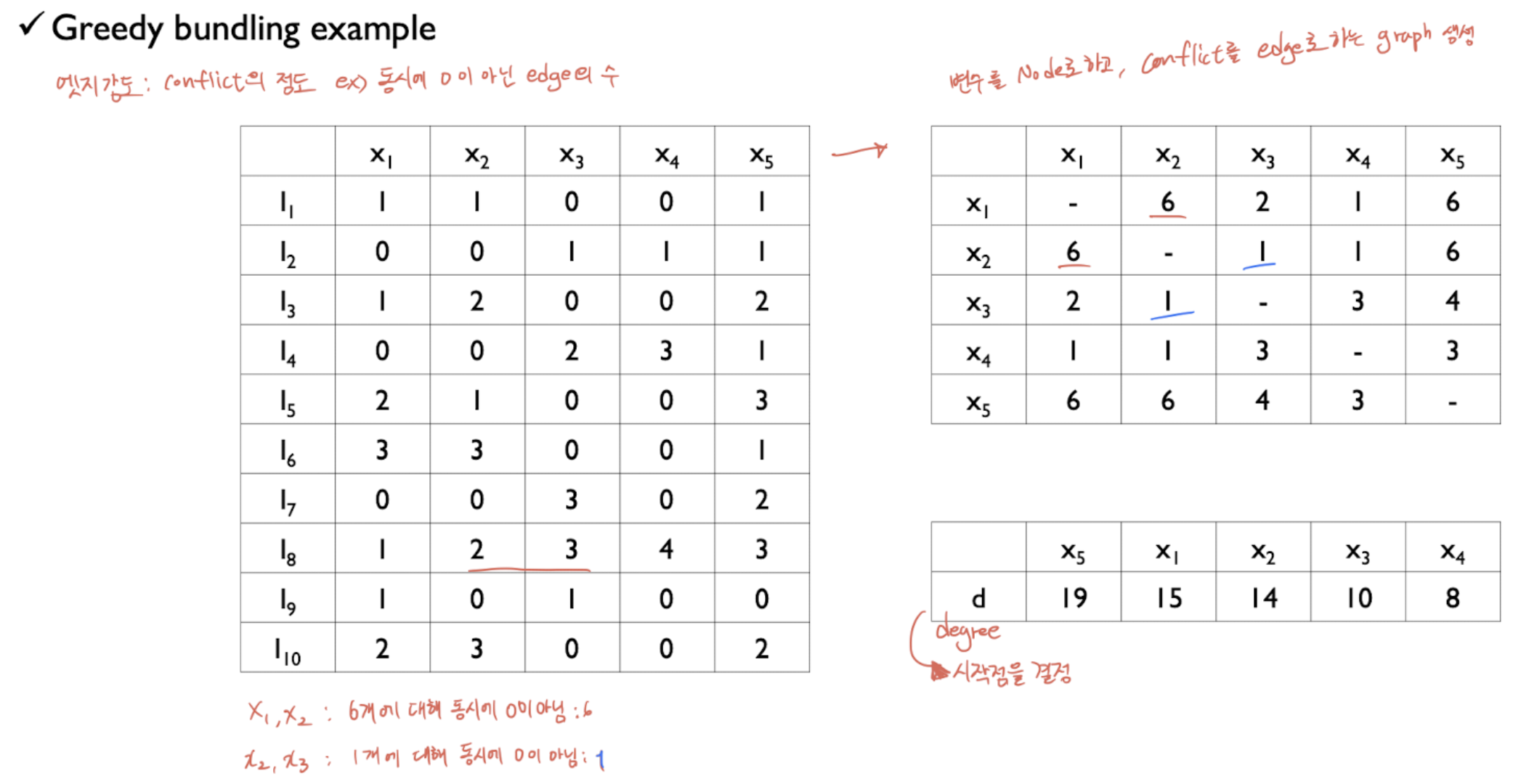
예를들어 이러한 데이터셋(x1~x5) 먼저 각각의 conflict를 Edge로 하는 Graph를 생성한다 (오른쪽 위)
여기서 conflict는 서로 상충하는 데이터 개수(동시에 0이 아닌 데이터 개수)이다.
이를 바탕으로 오른쪽 아래의 Degree를 계산할 수 있고, 이를통해 시작점을 계산한다. 위의 그림에서는 x5부터 시작.

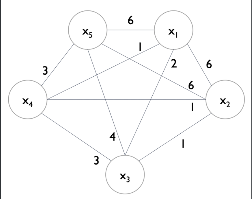
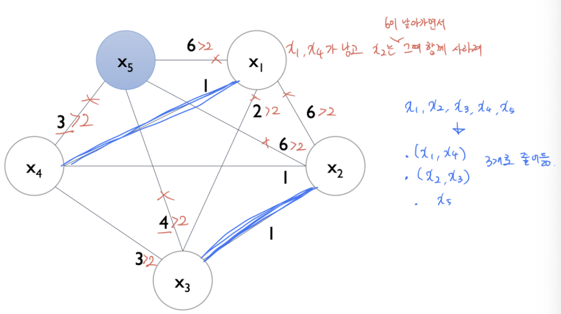
이렇게 그래프에서 x5부터 시작하며, 각각의 edge는 상충하는 데이터 개수(conflict)이다.
여기서 cut-off가 등장하는데, 이를 기준으로, 번들링에서 cut-off만큼 이상의 conflict라면, 하나의 번들로 묶지않는것이다.
위의 데이터에서는 10개 중 cut-off = 0.2로, 2개 이상 conflict 등장하면 엣지날림.
x5는 동떨어지게되므로 그대로가고,
x1을 계산할 때, x1과 x2는 6의 conflict로 날리고 x3도 날리면, ... x1,x4가 하나의 번들로 묶이게된다.
x2를 계산할 때, 이미 번들링된것을 제외하고, x3과 번들로 묶임. 더이상 묶을게 없으므로 종료.

이제 이렇게 묶은 번들에 대하여 Merge Exclusive Features를 진행한다.

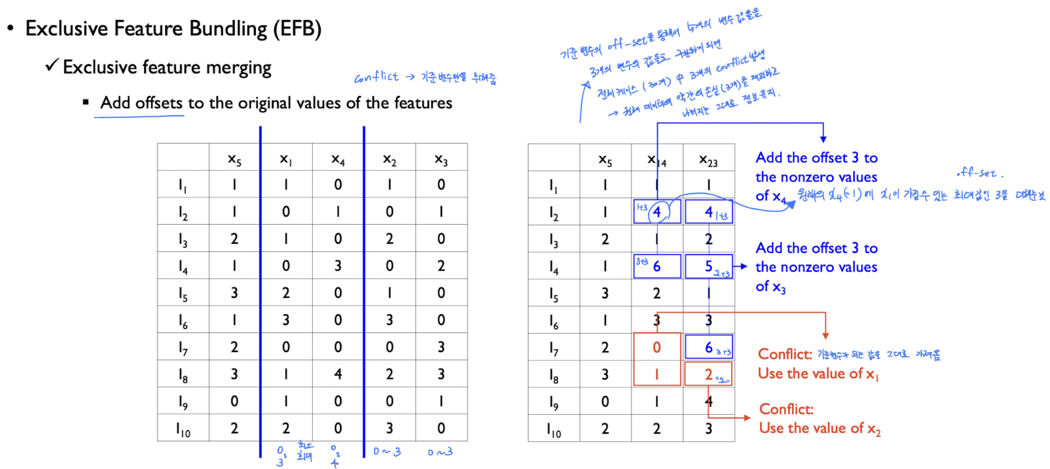
각각 column(feature)에 대해 cardinality처럼 최대와 최소값을 기록하고, 기준이 되는 feature에 함께묶인 feature와 merge를 해주는것이다.
이때, 기준값이 있다면 그대로 기준값을 사용하고, 기준값이 없다면, 기준feature의 최대값 + 묶인녀석의 값을 해서 넣게된다.
conflict한 경우(둘다 값이 있을 때 or 둘다 0일때) 기준값을 사용한다. (빨강 박스)

사용 예

사이킷런 사용

import lightgbm
lgbm = lightgbm.LGBMClassifier(n_estimators=1500, n_jobs=-1, 
                            #    scale_pos_weight=(0.888/0.111)  # Unbalanced한 데이터
                                is_unbalance=True # Unbalanced한 데이터
                               )
eval_set=[(X_train,y_train),(X_val,y_val)]
lgbm.fit(X_train,y_train, eval_set=eval_set,eval_metric='f1',verbose=50 ,early_stopping_rounds=100)
lgbpred = lgbm.predict(X_val)

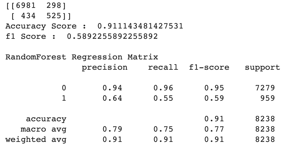
print(confusion_matrix(y_val, lgbpred))
print('Accuracy Score : ',accuracy_score(y_val, lgbpred))
print('F1 Score : ',f1_score(y_val, lgbpred))
print('\nRandomForest Regression Matrix\n' , classification_report(y_val, lgbpred))

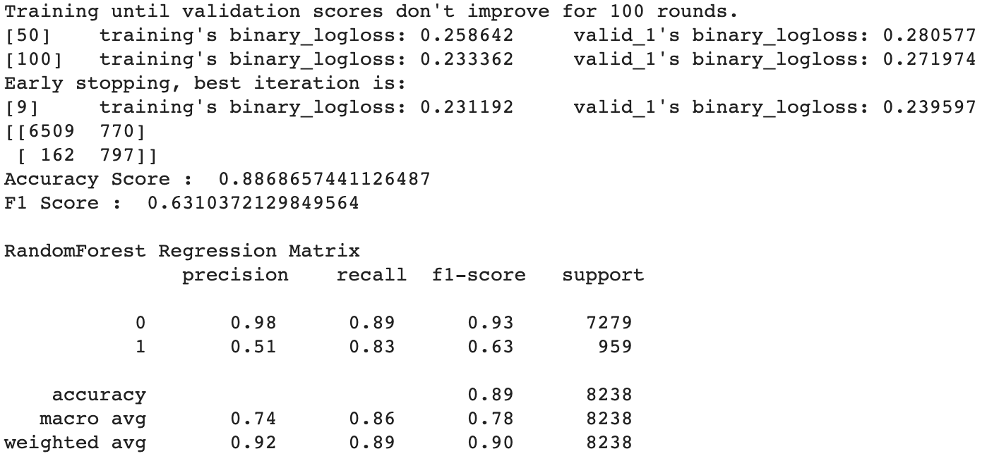
Parameter Tunning

BayesianOptimization

!pip install bayesian-optimization
from bayes_opt import BayesianOptimization

def bayesian_param_opt_lgb(X,y,init_round=15,opt_round=25,n_folds=5,random_seed=42,n_estimators=10000,learning_rate=0.05, output_process=False):
    train_data=lightgbm.Dataset(data=X_train, label=y)
    def lgb_eval(num_leaves, feature_fraction, bagging_fraction, max_depth, min_split_gain, min_child_weight):
        params={'application':'binary','num_iterations': n_estimators, 'learning_rate':learning_rate,'early_stopping_round':100,'metric':'auc'}
        params['num_leaves'] = int(round(num_leaves))
        params['feature_fraction'] = max(min(feature_fraction,1),0)
        params['bagging_fraction'] = max(min(bagging_fraction,1),0)
        params['max_depth'] = int(round(max_depth))
        params['min_split_gain'] = min_split_gain
        params['min_child_weight'] = min_child_weight
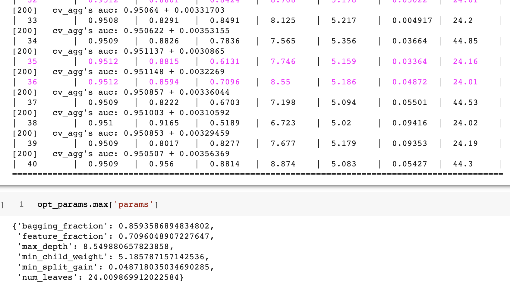
        cv_result=lightgbm.cv(params, train_data, nfold=n_folds,seed=random_seed, stratified=True, verbose_eval=200, metrics=['auc'])
        return max(cv_result['auc-mean'])
    lgbBO=BayesianOptimization(lgb_eval, {'num_leaves':(24,45),
                                          'feature_fraction':(0.1,0.9),
                                          'bagging_fraction':(0.8,1),
                                          'max_depth':(5,9),
                                          'min_split_gain':(0.001,0.1),
                                          'min_child_weight':(5,50)}, random_state=42)
    lgbBO.maximize(init_points=init_round, n_iter=opt_round)
    return lgbBO
opt_params=bayesian_param_opt_lgb(X_train,y_train)##,init_round=5, opt_round=10, n_folds=3, random_seed=42, n_estimators=100,learning_rate=0.05)

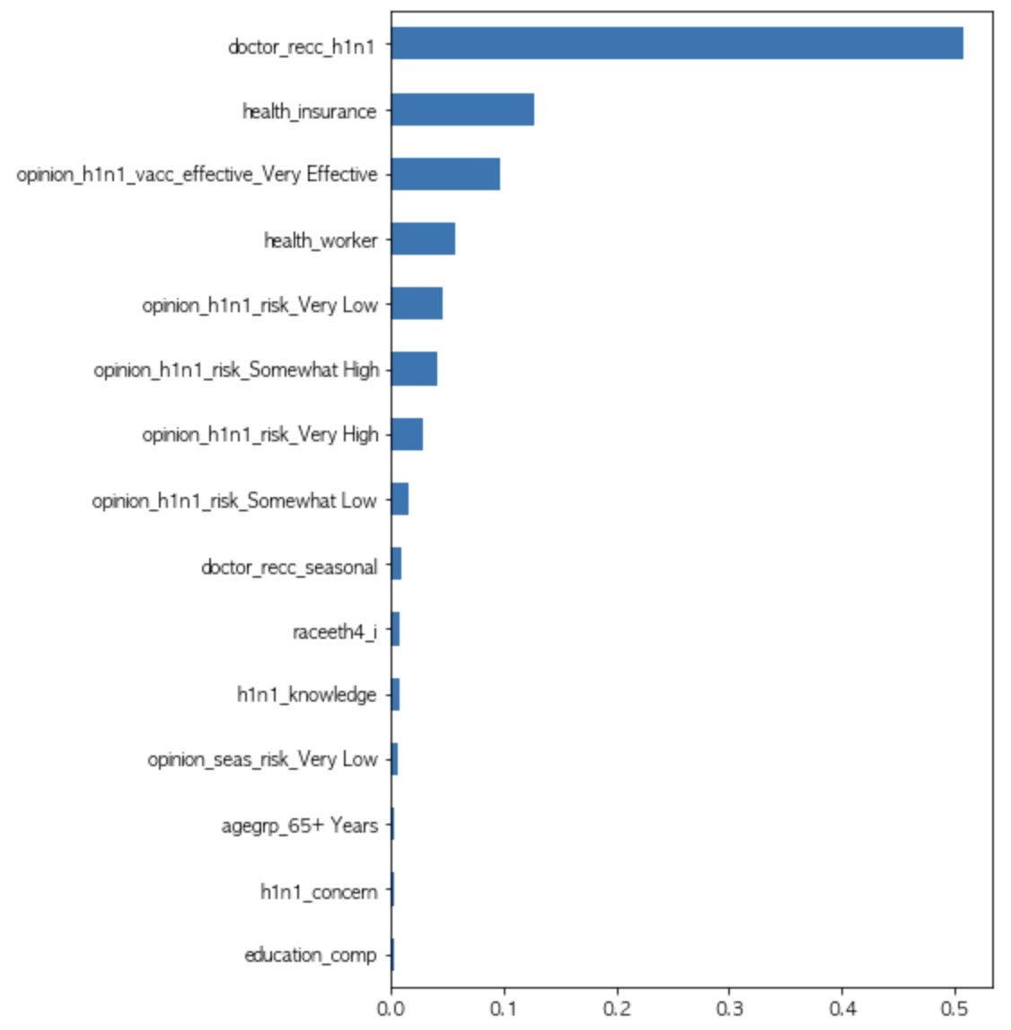
Featrue Importance를 확인해볼 수 있는 모듈을 제공한다.

from lightgbm import plot_importance
plot_importance(lgb_model)

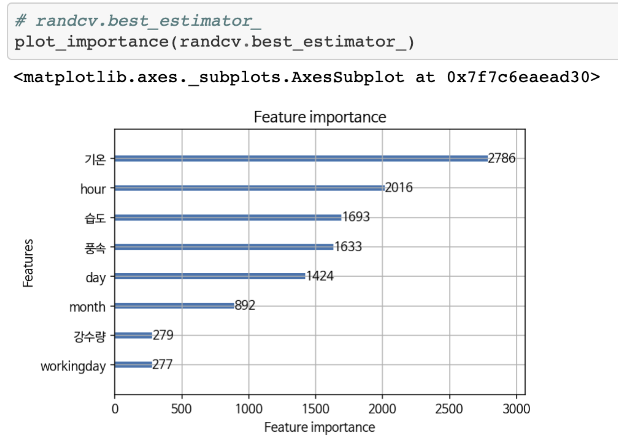
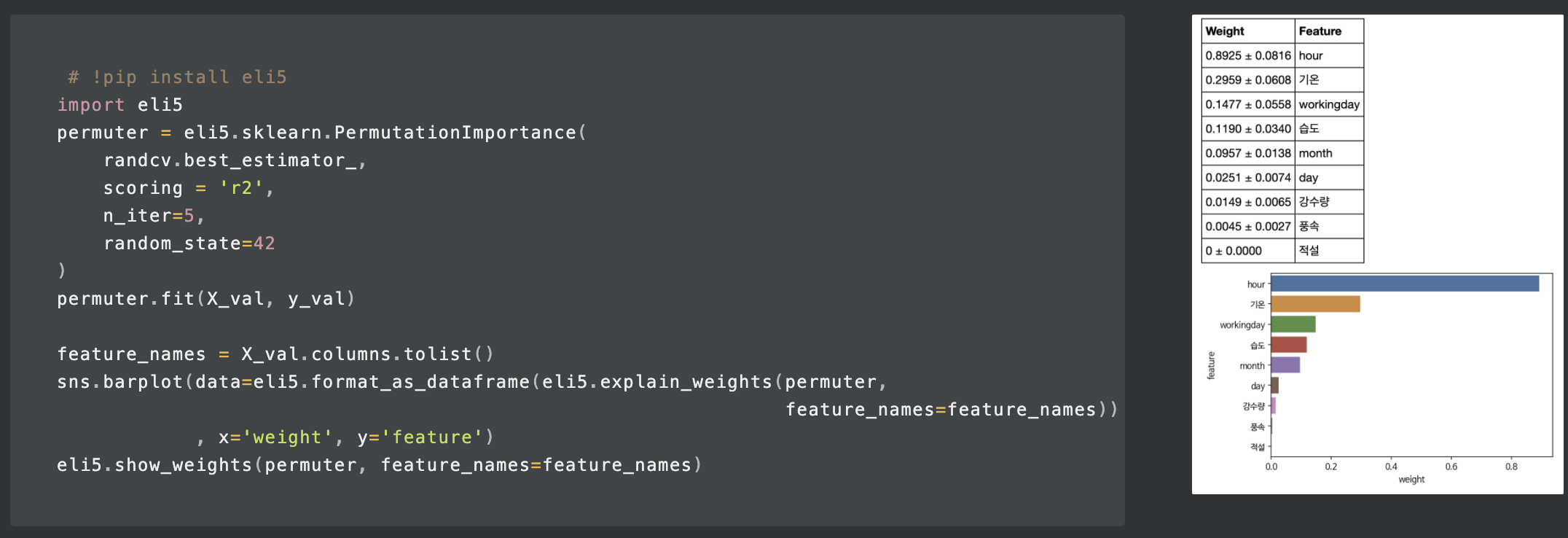
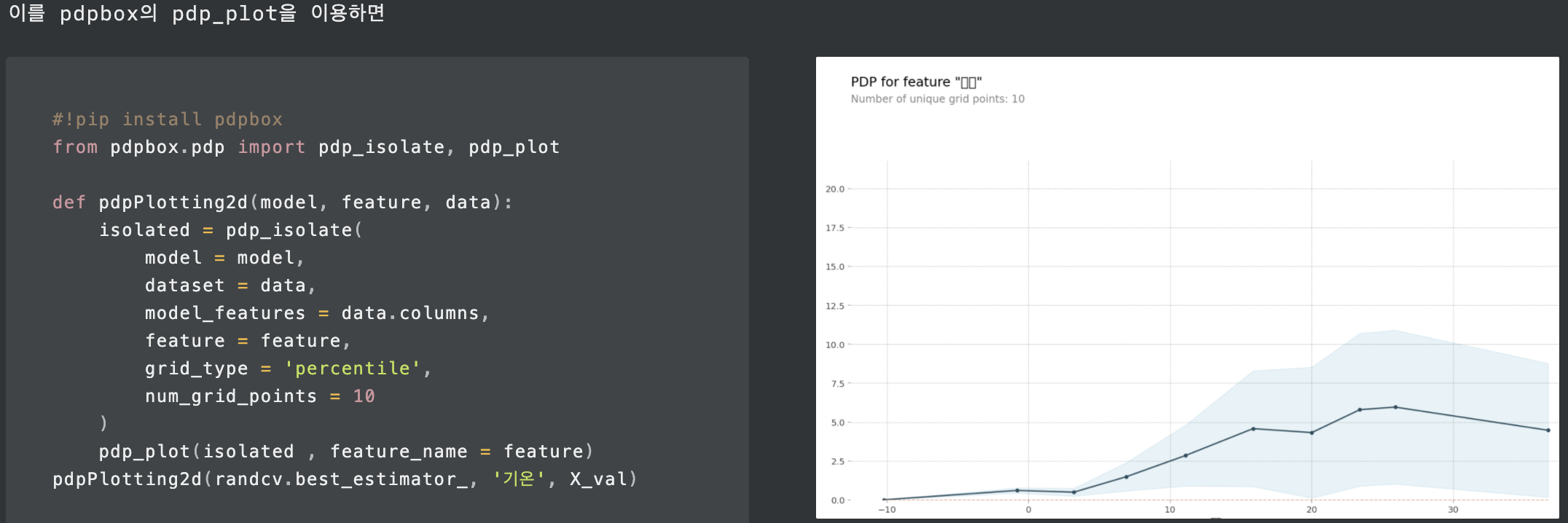
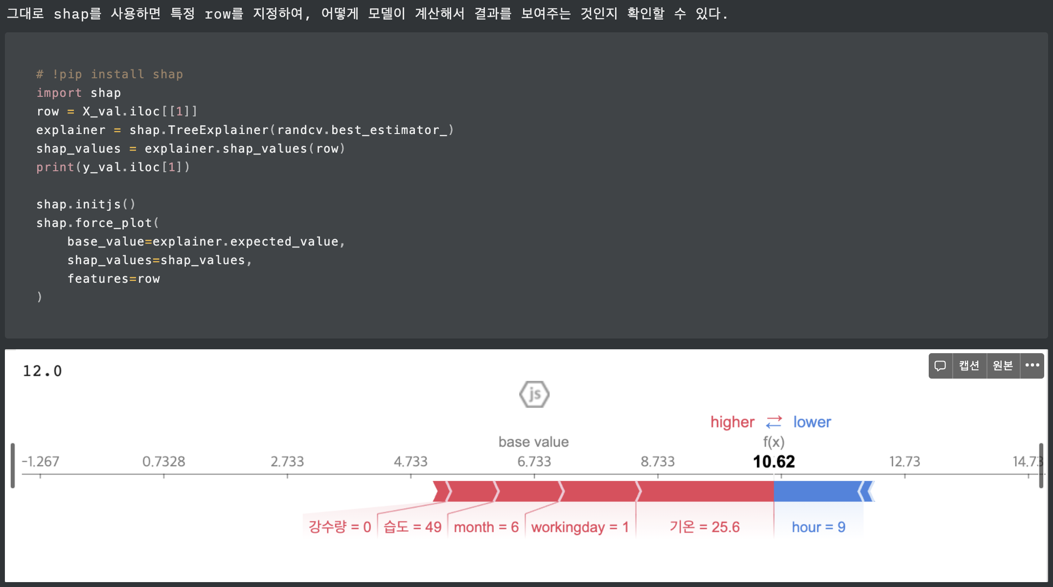
또한, eli5를 통해 Permutation Importance를 볼 수 있고, pdpbox의 pdp_plot, shap으로도 feature_importance를 볼 수 있다.

핵심 파라미터

max_depth : Tree의 최대 깊이를 말합니다. 이 파라미터는 모델 과적합을 다룰 때 사용됩니다. 만약 여러분의 모델이 과적합된 것 같다고 느끼신다면 제 조언은 max_depth 값을 줄이라는 것입니다.

min_data_in_leaf : Leaf가 가지고 있는 최소한의 레코드 수입니다. 디폴트값은 20으로 최적 값입니다. 과적합을 해결할 때 사용되는 파라미터입니다.

feature_fraction : Boosting (나중에 다뤄질 것입니다) 이 랜덤 포레스트일 경우 사용합니다. 0.8 feature_fraction의 의미는 Light GBM이 Tree를 만들 때 매번 각각의 iteration 반복에서 파라미터 중에서 80%를 랜덤하게 선택하는 것을 의미합니다.

bagging_fraction : 매번 iteration을 돌 때 사용되는 데이터의 일부를 선택하는데 트레이닝 속도를 높이고 과적합을 방지할 때 주로 사용됩니다.

early_stopping_round : 이 파라미터는 분석 속도를 높이는데 도움이 됩니다. 모델은 만약 어떤 validation 데이터 중 하나의 지표가 지난 early_stopping_round 라운드에서 향상되지 않았다면 학습을 중단합니다. 이는 지나친 iteration을 줄이는데 도움이 됩니다.

lambda : lambda 값은 regularization 정규화를 합니다. 일반적인 값의 범위는 0 에서 1 사이입니다.

min_gain_to_split : 이 파라미터는 분기하기 위해 필요한 최소한의 gain을 의미합니다. Tree에서 유용한 분기의 수를 컨트롤하는데 사용됩니다.

max_cat_group : 카테고리 수가 클 때, 과적합을 방지하는 분기 포인트를 찾습니다. 그래서 Light GBM 알고리즘이 카테고리 그룹을 max_cat_group 그룹으로 합치고 그룹 경계선에서 분기 포인트를 찾습니다. 디폴트 값은 64 입니다.

출처 :
LightGBM
Go Lab
고려대 일반대학원 산업경영공학과 비즈니스 애널리틱스 강의 (Pilsung Kang교수님)
파라미터튜닝
https://lsjsj92.tistory.com/548?category=853217
https://lightgbm.readthedocs.io/en/latest/Python-Intro.html#setting-parameters
http://machinelearningkorea.com/2019/09/25/lightgbm의-핵심이해/

eli5

Permutation Importance

각 특성의 값을 random하게 변형을 하고, 그 때 얼마나 error가 커지는지를 기준으로 각 특성의 중요도를 산출

!pip install eli5
import eli5
permuter = eli5.sklearn.PermutationImportance(
    xgbr, ## 이미 학습이 완료된 모델
    scoring = 'r2',
    n_iter=5,
    random_state=42
)
permuter.fit(X_val, y_val)
feature_names = X_val.columns.tolist()
sns.barplot(data=eli5.format_as_dataframe(eli5.explain_weights(permuter, feature_names=feature_names)), x='weight', y='feature')
eli5.show_weights(permuter, feature_names=feature_names)

pdpbox

Ensemble모델을 만들었을때 가장 큰 문제가 뭐냐함은, 이 모델의 성능은 알겠는데... 어찌 해석해야할지 난감할때가 많다는 것이다. 

Decision 트리를 제외하곤 세부과정들에서 만들어진 트리들을 하나하나 그려보거나 뜯어볼 수 없으니.. 이를 어떻게 확인할 것이냐. 라는 의문속에 많은 데싸인들이 고통받아왔다. 

pdpbox는 이를 해결하기 위해 나온 라이브러리이다. 

특성값에 따라 타겟값이 증가하는지, 감소하는지를 알 수 있다. 

이는 특성들을 선형적으로 변화시키면서 타겟이 어떻게 되는지를 보는것이다.

pdp에서는 최대 두 특성이 동시에 모델에 끼치는 영향을 볼 수 있으며 이를 통해 의존도를 볼 수 있다. 

아주 간단하다. 모델넣고, Validation Data넣고, 그 모델의 Feature들을 이름을 넣어주고나서 확인하고싶은 feature를 입력하면된다. 

#!pip install pdpbox
from pdpbox import pdp
feature = 'duration'
pdp_dist = pdp.pdp_isolate(model=xgb, dataset = X_val , model_features=X_val.columns, feature = feature)
pdp.pdp_plot(pdp_dist, feature)

features = ['age', 'education']
interaction = pdp.pdp_interact(
    model=xgb, 
    dataset=X_train, 
    model_features=X_train.columns, 
    features=features
)
pdp.pdp_interact_plot(interaction, plot_type='grid', feature_names=features, plot_params={'font_family':'NanumBarunGothic'});

shap

블랙박스와도 같은 모델을 투명하게 바꿔준다. 

게임이론에 나오는 shapely values에 기초하여 계산함. 

[모든 특성들을 조합했을 때 결과]에서 [관심있는 특성들을 제외한 조합]으로 계산된 결과를 뺀 값이 그 특성이 기여한 가치라고 판단. 

-> 그녀석이 없어지니 100점이 까였어 -> 그녀석의 기여도 ==100

데이터 특성 하나에 대한 설명 ->  개별 관측치 하나마다 특성의 영향도가 다르게 계산될 수 있음. 

plot type 을 bar로 주면, feature_importance_ 와 비슷하게, 특성의 영향력을 전체적으로 평가해줌. 

기존의 Permutation Importance (eli5)보다 정확하다. 그 이유는 특성중요도는 음의관계에 대하여 계산하지 않고, 서로 다른 특성들 간의 영향을 주는 경우 결과가 정확하지 않을 수 있기 때문이다. 

# !pip install shap
import shap
row=5
row = X_val.iloc[[9]]
explainer = shap.TreeExplainer(lgb_model)
shap_values = explainer.shap_values(row)
print(y_val.iloc[9])

shap.initjs()
shap.force_plot(
    base_value=explainer.expected_value, 
    shap_values=shap_values,
    features=row
)

출처 : 

pdpbox.readthedocs.io/en/latest/

github.com/SauceCat/PDPbox

분류를 하는 모델에서의 모델의 성능을 평가하는 방법을 소개합니다.

혼동행렬 Confusion Matrix

분류작업에서 사용하며, Matrix로 그려볼 수 있음.
ex) 스팸메일 100개 중 실제 스팸메일이 60개인 상황에서, 어떠한 모델의 스팸분류결과 스팸메일:80개가 나왔고 , 그중 55개가 진짜 스팸메일인 경우
이를 표로 나타내면

위와 같은 혼동행렬을 얻을 수 있다.

여기서 중요한 개념이 등장하는데 TP, FP, FN, TN 이다.

• TP ( True Positive ) : (모델이) 양성판단했는데, 실제로도 양성인경우 -> 양성판단으로 맞은경우
• TN ( True Negative ) : (모델이) 음성판단했는데, 실제로도 음성인경우 -> 음성판단으로 맞은경우
• FP ( Flase Positive ) : (모델이) 양성판단했는데, 실제로는 음성인경우 (틀린경우) -> 양성판단으로 틀린경우
• FN ( Flase Negative ) : (모델이) 음성판단했는데, 실제로는 양성인경우 (틀린경우) -> 음성판단으로 틀린경우

Precision (정밀도)

$$ TP \over {TP + FP}$$
양성 예측이 정답을 정확히 예측한 비율

분류결과 스팸메일(양성판단)로 나온 80개 중 실제 스팸메일피 55개 이므로 위의 경우 정밀도는 $5 \over {55+25} $ 이다.

Recall (재현률)

$$ TP \over {TP + FN}$$
실제로 양성인녀석들 중 모델에서 양성으로 판단한 비율

실제 스팸메일(양성) 60개 중 스팸메일로 분류(양성판단)을 받은 55개에 해당하므로 재현률은 $ 55 \over {55+5}$ 이다.

Accuracy (정확도)

$$ {TP + TN}\over{TP+TN+FP+FN}$$
전체 중 (양성 판단이든 음성 판단이든)맞은 비율

전체 메일 100개 중 스팸으로 맞게 분류된 55개의 스팸메일 , 일반메일로 맞게 분류된 15개의 일반메일 : $ {55+15}\over{100}$

F1 Score

정밀도와 재현률의 상충관계를 평가에 반영하여 조화평균한 점수이다.
대부분의 분류문제에서 데이터의 분포에 차이가 있는 경우가 많으므로 주로 F1 Score를 사용하는 경우가 많다.

만약 잘못 판정해서는 안되는 문제에서 예를들면, '정밀도 0.9 미만의 모델은 채용하지 않는다'라는 최소 조건을 정하고, 이 조건을 만족하면서 F1 Score가 높아지도록 파라미터를 튜닝한 다음 모델을 선택하면 된다.

AUC , ROC

ROC (Receiver Operating Characteristic : 수신자 조작 특성) : 모든 임계값에서 분류 모델의 성능을 보여주는 그래프

AUC (Area Under the Curve) : ROC 곡선 아래의 영역

AUC가 높다는 것은 클래스를 구벼라는 모델의 성능이 훌륭하다는 것을 의미한다. 

Sensitivity 민감도  :  기존의 Precision과 같다. 실제 스팸일때, 모델결과도 스팸인경우

Specificity 특이도 : 실제 스팸이 아닐때, 모델결과도 스팸이 아니라고 나오는경우

Positive Likelihood ratio : 양성우도비 : 실제 스팸일때, 모델결과 스팸일 확률과, 실제 스팸이아닐때(일반), 모델결과가 스팸일 확률 사이의 비율

$$ {{ {True Positive Rate}\over {False Positive Rate} } }= {{Sensitivity}\over{1-Specificity}}$$

Negative Likelihood ratio : 음성우도비 : 실제 스팸일때 모델결과 일반메일일 확률과 실제 일반메일이 모델결과도 일반일 확률의 비율

$$ {{ {False Negative Rate}\over {True Negative Rate} } }= {{1-Sensitivity}\over{Specificity}}$$

Positive Predictive Value : 양성예측도 : 모델결과 스팸판정일때, 진짜로 스팸이었을 확률 

Negative Predictive Value : 음성예측도 : 모델결과 일반판정일 때, 실제로 일반메일일 확률

___

from sklearn.metrics import roc_curve
from sklearn.metrics import roc_auc_score

# roc_curve(타겟값, prob of 1)
# fpr, tpr, thresholds = roc_curve(y_val, y_pred_proba)

base_prob=[0 for i in range(len(y_val))]
logit_prob[:,1]
grid_best_pipe_prob[:,1]
rand_best_pipe_prob[:,1]

# AUC
base_auc = roc_auc_score(y_val,base_prob)
logit_auc = roc_auc_score(y_val, logit_prob[:,1])
grid_auc = roc_auc_score(y_val, grid_best_pipe_prob[:,1])
rand_auc = roc_auc_score(y_val, rand_best_pipe_prob[:,1])

#Curve
base_fpr, base_tpr, _ = roc_curve(y_val,base_prob)
logit_fpr, logit_tpr, _ = roc_curve(y_val, logit_prob[:,1])
grid_fpr, grid_tpr, _ = roc_curve(y_val, grid_best_pipe_prob[:,1])
rand_fpr, rand_tpr, thresholds = roc_curve(y_val, rand_best_pipe_prob[:,1])


plt.figure(figsize=(8,8))
plt.plot(base_fpr, base_tpr, linestyle='-', label='Baseline')
plt.plot(logit_fpr, logit_tpr, marker='.', label='Logistic')
plt.plot(grid_fpr, grid_tpr, marker='.', label='GridSearchCV _ Best')
plt.plot(rand_fpr, rand_tpr, marker='.', label='RandomSearchCV _ Best')
plt.legend();plt.grid();plt.xlabel('FPR');plt.ylabel('TPR');plt.show()

아주 미세하게 RandomSearchCV_Best가 좀 더 큰값을 갖고있음을 알 수 있으며, 이는 더욱 높은 성능을 보인다고 할 수 있다.

Thresholds

넘파이의 argmax함수를 이용하면 최대값의 인덱스를 뽑을 수 있다. 여기서 fpr - tpr 를 최대로 하는 것을 찾으면 

# threshold 최대값의 인덱스, np.argmax()
optimal_idx = np.argmax(rand_tpr - rand_fpr)
optimal_threshold = thresholds[optimal_idx]

print('idx:', optimal_idx, ', threshold:', optimal_threshold)
#idx: 512 , threshold: 0.3868291239669877

Threshold : 0.387 에서 tpr-fpr의 최대값을 찾을 수 있는데, 

이것을 활용하여 새로 Classification Report를 만들어보면 

#사용하지 않은 일반모드
print( " 0.5 사용")
y_pred_optimal = rand_best_pipe_prob[:,1] >= 0.5
print(classification_report(y_val, y_pred_optimal))

# Optimal Threshold 사용한 모드'
print( " Threshold 사용")
y_pred_optimal = rand_best_pipe_prob[:,1] >= optimal_threshold
print(classification_report(y_val, y_pred_optimal))

위와같은 형태로 Accuracy는 조금 감소하지만 class 1의 f1 score와 recall을 증가시킬 수 있다. 

그럼 여기서 Threshold 0.5와 0.62가 어떤 의미를 갖는지 보자. 

fig, axes=plt.subplots(1,2, figsize=(18,8))
axes[0].axvline(optimal_threshold,color="red")
axes[1].axvline(0.5,color="red")
sns.histplot(rand_best_pipe_prob,bins=200,ax=axes[0] ).set_title('RandomSearchCV _ Optimal Threshold :: 0.38')
sns.histplot(rand_best_pipe_prob,bins=200,ax=axes[1] ).set_title('RandomSearchCV _ Threshold 0.5')
plt.show()

predict_prob() 함수를 통하여 각 클래스의 판별 확률을 plot하여 선을 그었다.

이게 무슨뜻이냐함은, Threshold값을 기준으로 왼쪽은 1, 오른쪽은 0 으로 판단했다는 것이며 Threshold값이 

왼쪽그림은 Optimal Threshold 인 0.38을 기준으로 했을때이고, 오른쪽은 baseline인 0.5를 기준으로 했을때 이다. 

0으로 판별받는녀석이 많아지고, 1로 판별받는 녀석이 더 적어진다. -> 진짜 1인녀석들이 남을 가능성이 높아지는것 -> recall이 높아지는것

Threshold값을 통하여, 분류에서 예측값의 클래스 확률값을 통하여 조절을 할 수 있다는것이다. 

참조 : arifromadhan19.medium.com/part-1-regression-and-classification-model-evaluation-bc7f6ab3b4dd

datascienceschool.net/03%20machine%20learning/09.04%20%EB%B6%84%EB%A5%98%20%EC%84%B1%EB%8A%A5%ED%8F%89%EA%B0%80.html?highlight=auc

정확도 (Accuracy)

아주 직관적이며 간단하다
$정확도 = {{정답과 일치한 수}\over{전체 데이터 수}} = {{TP + TN} \over {Total}} $
전체 범주를 모두 바르게 맞춘 경우를 전체 수로 나눈값이다.

정밀도 (Precision) : Positive로 예측한 것 중 올바른것

$정밀도 = {TP \over {TP+ FP} }$

재현율 (Recall) : 실제 Positive 중 올바르게 positive를 맞춘 것의 비율

$ 재현율 = {TP\over{TP+FN}}$

F1_score : 정밀도(Precision)와 재현율(Recall)의 조화평균

${F-점수} = { 2 \over { {1\over정밀도}+{1\over재현율}}} = {2*{Precision * Recall \over {Precision + Recall}}}$

Confusion Matrix

(Example)

from sklearn.metrics import plot_confusion_matrix

fig, ax = plt.subplots()
pcm = plot_confusion_matrix(grid_best_pipe, X_val, y_val,
                            cmap=plt.cm.Blues,
                            ax=ax);
plt.title(f'Confusion matrix, n = {len(y_val)}', fontsize=15)
plt.show()

cm = pcm.confusion_matrix
correct_pred = np.diag(cm).sum()
total_pred = cm.sum()
print(f'[TP , TN] : {np.diag(cm)}') # TP + TN
print(f' TP + TN (정확하게 맞춘 예측) : {correct_pred}')
print(f' 총 예측 수 : {total_pred}')
print(f' 분류정확도 (Accuracy) : {round(correct_pred/total_pred,3)}')
print(f' Accuracy함수 accuracy_score : {round(grid_best_pipe.score(X_val,y_val),3)}')
print()     # 실제     기계
tp=cm[1][1] # 맞는걸   맞다해 
fn=cm[1][0] # 맞는데   틀렸데 
fp=cm[0][1] # 틀렸는데  맞았데 
tn=cm[0][0] # 틀린걸   틀렸다해 
print(f'정밀도 (Precision) : {tp/(tp+fp)}') # TP / TP + fP
print(f'재현률 (Recall) : {tp/(tp+fn)}') # TP / TP + fP

[TP , TN] : [2990  560]
 TP + TN (정확하게 맞춘 예측) : 3550
 총 예측 수 : 4214
 분류정확도 (Accuracy) : 0.842
 Accuracy함수 accuracy_score : 0.842

정밀도 (Precision) : 0.6306306306306306
재현률 (Recall) : 0.625

sklearn의 metrics의 모듈을 통해 혼동행렬을 만들어보았다.

Ensemble 학습의 Bagging 의 대표적인 방식

앙상블이랑 여러개의 알고리즘을 사용하여, 그 예측을 결정함으로써 보다 정확한 예측을 도출하는 기법.

기존의 Decision Tree에서 그 트리가 엄청많아져서, 그것들의 최종 값의 비율로 계산하자!

각각 부트스트랩으로 만들어진 데이터셋으로 학습하게되는데, 이를 Bagging (Bootstrap AGGregatING) 이라고 한다.

오리지널 데이터에서 복원추출하는데, 샘플을 뽑고, 다시 원본에서 샘플을 뽑는다. (중복될 수 있다는것)
원본 데이터셋에서 복원추출하는 것을 Bootstrap Sampling이라 한다.
그렇게 samples들을 뽑아서 원본과 같은 수의 sample을 구성하면 그게 부트스트랩샘플을 하나 만들었다고 한다.
각각의 부트스트랩 샘플의 Training set 에서 뽑히지 않은 샘플들을 test set으로 분류하고 이를 OOB Sample이라고 한다.
→ 100 개 데이터 중 70개로 트레인하고, 나머지 30개로 validation을 매 트리 생성시마다 한다고 보면 됨.

앙상블 기법은 한 종류의 데이터로 여러 학습모델을 만들어, 그 모델들의 예측결과를 다수결이나 펴균을 내어 예측하는 방법을 말한다.

랜덤포레스트는 Decision Tree를 기본모델로 사용한다.

부트스트랩 세트의 크기가 n일 때, 한번의 추출에서 어느 한 샘플이 추출되지 않을 확률은 ${n-1} \over n$ 이다. 
그것을 n번 반복였을 때에도 그 샘플이 추출되지 않았을 확률은 $ ({{n-1}\over n})^2$ 이다.
이게 이제 무한히 커지면 어느 한 점으로 수렴하게 되는데.

결과적으로 데이터가 충분할 때 한 부트스트랩 세트는 63.2%의 샘플을 갖고, 
여기에 속하지 않은 36.8% 의 샘플이 Out-of_Bag 샘플이며, 이것이 검증에 사용된다.

트리모델에서는 One-hot Encoding보다 Ordinal Encoding이 좀더 성능이 좋을 때가 많다.
원핫으로 피쳐가 추가되었을 때, 트리에서는 상위노드에서 중요한 피처가 사용되므로, 하나의 피쳐가 여러개의 피쳐로 쪼개진 One-Hot에서 범주 종류가 많은 (High Cardinality) 피쳐였을 경우 상위노드에서 선택될 가능성이 적어진다.

• n_estimators = 트리의 갯수 | number of trees in the foreset
• max_features = 노드들 구분할 때 고려할 최대 피쳐수 | max number of features considered for splitting a node
• max_depth = 각 트리의 최대 깊이 | max number of levels in each decision tree
• min_samples_split = 최소 분할 샘플 갯수 | min number of data points placed in a node before the node is split
• min_samples_leaf = 최소 잎 노드 데이터 수 | min number of data points allowed in a leaf node
• bootstrap = 복원 추출 | method for sampling data points (with or without replacement)

랜덤 포레스트의 Pseudo Code

S는 트레이닝셋, Feature 는 F, 랜덤포레스트 안의 트리는 B 라고 한다.
H를 초기화하고, 
1부터 B까지 (트리들을 순회하면서),
$S^(i)$ 에 S로 부터 만든 부트스트랩 샘플을 넣고, 
$h_i$ 에 트리를 학습시키고(트리의 학습은, 각각의 노드에서 feature의 subset을 최적으로 쪼개면서 학습시킨다. ), 
이후, 학습된 트리들 하나하나를 H에 합친 후, 최종 H를 리턴. 

from sklearn.model_selection import train_test_split

train, val = train_test_split(train, train_size=0.8, test_size=0.2,
                              stratify=train[target], random_state=2)
                              
##############################################                              
from category_encoders import OrdinalEncoder
from sklearn.pipeline import make_pipeline

pipe_ordinal_simple=make_pipeline(verbose=0,
    OrdinalEncoder(verbose=0),
    SimpleImputer(),
    RandomForestClassifier(n_jobs=-1, random_state=10, oob_score=True)
)

pipe_ordinal_simple.fit(X_train,y_train)
pipe_ordinal_simple.score(X_val,y_val) #0.8258806784485826

ㅇ 이렇게 파이프라인속에 넣어서 사용할 수도 있다. 
X_train으로 fit(학습)시키고, X_val로 분리해놓은 데이터를 통하여 점수를 매겨보는 등의 작업을 하면된다. 

하이퍼파라미터 튜닝

• n_estimators = 트리의 갯수 | number of trees in the foreset
• max_features = 노드들 구분할 때 고려할 최대 피쳐수 | max number of features considered for splitting a node
• max_depth = 각 트리의 최대 깊이 | max number of levels in each decision tree
• min_samples_split = 최소 분할 샘플 갯수 | min number of data points placed in a node before the node is split
• min_samples_leaf = 최소 잎 노드 데이터 수 | min number of data points allowed in a leaf node
• bootstrap = 복원 추출 | method for sampling data points (with or without replacement)
• class_weight =  sample의 라벨 비율 ->  기존의 분류문제에서 라벨비율이 비슷하지 않으면, 좋지 않은 학습결과를 가져올 수 있는데, 이를 처리해줌.

class_weight 설정

어떠한경우 target 의 class 비율이 다를 수 있다. 이는 모델 학습에 악영향을 끼치는데, 이 부분에 대하여 RandomForest에서는 class_weight라는 파라미터를 준다. 

from sklearn.utils.class_weight import compute_class_weight
print(y_train.unique(),'\n',y_train.value_counts())
compute_class_weight(class_weight='balanced', classes = y_train.unique(), y=y_train)
# [0 1] 
# 0    29269
# 1     3681
# Name: y, dtype: int64
# array([0.56288223, 4.47568595])
## _____________________ ## 
from sklearn.ensemble import RandomForestClassifier
rfc = RandomForestClassifier(n_estimators=250, class_weight={1:0.56288223 , 0:4.47568595})
rfc.fit(X_train, y_train)
rfcpred = rfc.predict(X_val)

print(confusion_matrix(y_val, rfcpred))
print('Accuracy Score : ',accuracy_score(y_val, rfcpred))
print('f1 Score : ',f1_score(y_val, rfcpred))
print('\nRandomForest Regression Matrix\n' , classification_report(y_val,rfcpred))

이를 통하여 불균형한 데이터 셋에서 Upsampling과 Downsampling하지 않고도 주어진 데이터를 최선으로 활용하여 학습을 진행할 수 있다. 

Max_depth 튜닝

def pipe_ordinal_simple_elbow(howmany,X_train, y_train, X_val, y_val):
    trainAccuracy=[]
    valAccuracy=[]
    for depth in range(1,howmany):
        pipe_ordinal_simple=make_pipeline(
            OrdinalEncoder(verbose=0),
            SimpleImputer(),
            RandomForestClassifier(max_depth=depth,n_jobs=-1, random_state=10, oob_score=True)
        )
        pipe_ordinal_simple.fit(X_train,y_train)
        trainAccuracy.append(pipe_ordinal_simple.score(X_train,y_train))
        valAccuracy.append(pipe_ordinal_simple.score(X_val,y_val))
    return trainAccuracy, valAccuracy
ta_msl , tv_msl = pipe_ordinal_simple_elbow(howmany=20 , 
                                             X_train=X_train,
                                             y_train=y_train, 
                                             X_val=X_val, 
                                             y_val=y_val)
                                             
pd.DataFrame({'msl_training': ta_msl, 'msl_val':tv_msl}, index=range(1,20)).plot(figsize=(10,8))
plt.grid()

depth 가 7~8을 넘어가는 부분부터 training과 validation의 accuracy score가 확연히 달라진다. 
깊어질수록 training은 정확도가 높아지는반면, val의 정확도는 거의 변하지않는다. 이는 과적합되는 부분이라고 봐도 될것이다.

n_estimator

n_estimators = 트리의 갯수 | number of trees in the foreset
한마디로 투표용지의 개수가 얼마나 많아지는가? 라고 생각하면 된다. 

def pipe_ordinal_simple_elbow_estimators(howmany,X_train, y_train, X_val, y_val):
    trainAccuracy=[]
    valAccuracy=[]
    for depth in range(10,howmany, 20):
        pipe_ordinal_simple=make_pipeline(
            OrdinalEncoder(verbose=0),
            SimpleImputer(),
            RandomForestClassifier(n_estimators=depth,n_jobs=-1, random_state=10, oob_score=True)
        )
        pipe_ordinal_simple.fit(X_train,y_train)
        trainAccuracy.append(pipe_ordinal_simple.score(X_train,y_train))
        valAccuracy.append(pipe_ordinal_simple.score(X_val,y_val))
    return trainAccuracy, valAccuracy
ta_msl , tv_msl = pipe_ordinal_simple_elbow_estimators(howmany=200 , 
                                             X_train=X_train,
                                             y_train=y_train, 
                                             X_val=X_val, 
                                             y_val=y_val) 
                                             
pd.DataFrame({'msl_training': ta_msl, 'msl_val':tv_msl}, index=range(10,200,20)).plot(figsize=(10,8))
plt.grid()

시작을 10부터 잡아서 그런지, 거의 변화가 너무 적다. 하지만 확실하게 1부터 시작한다면 증가하는 폭을 볼 수 있을것이다.

GridSearchCV 를 통한 하이퍼파라미터 튜닝

from sklearn.model_selection import GridSearchCV

params = { 'randomforestclassifier__n_estimators' : [50, 100, 150],
           'randomforestclassifier__max_depth' : [6, 9, 12],
           'randomforestclassifier__min_samples_leaf' : [8, 12],
           'randomforestclassifier__min_samples_split' : [8, 16]
            }
pipe_ordinal_simple=make_pipeline(
            OrdinalEncoder(verbose=0),
            SimpleImputer(),
            RandomForestClassifier(n_jobs=-1, random_state=10, oob_score=True)
        )
grid=GridSearchCV(pipe_ordinal_simple , param_grid=params , cv=5, verbose=0)
grid.fit(X_train,y_train)
grid.best_estimator_

Pipeline(steps=[('ordinalencoder',
                 OrdinalEncoder(cols=['opinion_h1n1_vacc_effective',
                                      'opinion_h1n1_risk',
                                      'opinion_h1n1_sick_from_vacc',
                                      'opinion_seas_vacc_effective',
                                      'opinion_seas_risk',
                                      'opinion_seas_sick_from_vacc', 'agegrp',
                                      'employment_status', 'census_msa',
                                      'state'],
                                mapping=[{'col': 'opinion_h1n1_vacc_effective',
                                          'data_type': dtype('O'),
                                          'mapping': Somew...
TENNESSEE              39
FLORIDA                40
NEW HAMPSHIRE          41
IDAHO                  42
MAINE                  43
ALASKA                 44
WISCONSIN              45
OKLAHOMA               46
MASSACHUSETTS          47
NORTH DAKOTA           48
WASHINGTON             49
NEBRASKA               50
HAWAII                 51
NaN                    -2
dtype: int64}])),
                ('simpleimputer', SimpleImputer()),
                ('randomforestclassifier',
                 RandomForestClassifier(max_depth=12, min_samples_leaf=12,
                                        min_samples_split=8, n_estimators=150,
                                        n_jobs=-1, oob_score=True,
                                        random_state=10))])

이러한 출력을 볼 수 있다. 

이제 이 파라미터들의 상태를 시각화해본다

cols='param_randomforestclassifier__max_depth param_randomforestclassifier__min_samples_leaf	param_randomforestclassifier__min_samples_split	param_randomforestclassifier__n_estimators mean_test_score'.split()
griddf=pd.DataFrame(grid.cv_results_)
fig,axs=plt.subplots(2,2, figsize=(10,10))
sns.pointplot(ax=axs[0][0], data=griddf, x=cols[0],y=cols[-1])
sns.pointplot(ax=axs[0][1], data=griddf, x=cols[1],y=cols[-1])
sns.pointplot(ax=axs[1][0], data=griddf, x=cols[2],y=cols[-1])
sns.pointplot(ax=axs[1][1], data=griddf, x=cols[3],y=cols[-1])

max_depth의 변화에 가장 크게 증가하였으며, 그외에는 오히려 조금 떨어진 경우가 많았다. 

Feature Importance

plt.figure(figsize=(4,8), dpi=110)
sns.barplot(data=
            pd.DataFrame(grid.best_estimator_['randomforestclassifier'].feature_importances_,
                         index=X_train.columns, columns=['feature_importances_']).reset_index().sort_values('feature_importances_',ascending=False)
                         , x='feature_importances_', y='index')

결정트리모델은 특성들을 기준으로 샘플을 분류해 나가는데, 마치 Tree model처럼 뻗어나간다고해서 Decision Tree라는 이름을 갖는다.

결정트리는 학습 결과로 IF-THEN 형태의 규칙이 만들어진다.

결정트리는 퍼셉트론이나 로지스틱 회귀와 달리 선형 분리 불가능한 데이터도 분류할 수 있으나, 선형분리 가능한 문제는 잘 풀지 못한다. 또한 데이터를 조건 분기로 나눠가는 특성상, 트리가 깊어질수록 학습에 사용되는 데이터 수가 적어져 과적합을 일으키기 쉽다.

결정 트리는 학습 데이터로부터 조건식을 만들고, 예측할 때는 트리의 루트(최상위조건)부터 순서대로 조건분기를 타면서 리프에 도착하면 예측결과를 내는 알고리즘이다.

불순도(Impurity)를 기준으로 가능한 한 같은 클래스끼리 모이도록 조건 분기를 학습한다.

구체적으로는 정보획득(Information Gain)이나 지니게수(Gini Coefficient)등의 값을 불순도로 사용해, 그 값이 낮아지도록 데이터를 분할한다.

이후 결정트리가 응용되어 랜덤포레스트와 경사부스팅결정트리가 생겨났다.

결정트리의 각 노드는 뿌리, 중간, 말단 노드로 나뉠 수 있다.

지니불순도

※ 지니계수 : 경제학에서 불평등지수를 나타낼 때 사용하는 것으로 0일 때 완전 평등, 1일 때 완전 불평등을 의미합니다.

머신러닝에서는 데이터가 다양한 값을 가질수록 평등하며 특정 값으로 쏠릴 때 불평등한 값이 됩니다. 즉, 다양성이 낮을수록 균일도가 높다는 의미로 1로 갈수록 균일도가 높아 지니계수가 높은 속성을 기준으로 분할

임의의 새로운 변수가 데이터셋으로부터 클래스 라벨의 분포를 따라 무작위로 분류된 경우, 임의 변수의 새로운 인스턴스의 잘못된 분류 가능성에 대한 측정치.
분류가 잘 되었는지 판단할 수 있는 척도이다.
$G_i = {1 - \Sigma_{k=1}^n{p_ik^2} }$

$I_G(p) = \Sigma_{i=1}^J{p_i ( 1-p_i) } = 1 - \Sigma_{i=1}^J{p_i^2} $
정보획득은 특정한 특성을 사용해 분할했을 떄 엔트로피의 감소량을 뜻한다.

여기서 불순도(impurity) 라는 개념은 여러 범주가 섞여 있는 정도를 이야기 한다.
예를들어 A, B 두 클래스가 혼합된 데이터가 있을 때 (A, B) 비율이 (45%, 55%)인 샘플(두 범주 수가 비슷)은 불순도가 높은 것이며
(80%, 20%)인 샘플이 있다면 상대적으로 위의 상태보다 불순도가 낮은 것 입니다. (순수도(purity)는 높음)

엔트로피

${\displaystyle \mathrm {H} (T)=\operatorname {I} _{E}\left(p_{1},p_{2},...,p_{J}\right)=-\sum _{i=1}^{J}{p_{i}\log _{2}p_{i}}}$

불순도를 측정하는 지표로서, 정보량의 기댓값.

$Entropy(S) = \Sigma_{i=1}^c{p_i * I(x_i)}$

S : 이미 발생한 사건의 모음 , c: 사건의 개수

정보량이란? :: 어떤 사건이 갖고있는 정보의 양을 의미하며, $I(x) = \log_2{1\over{p(x)}}$ 이다.

여기서 $p(x) : 사건이 발생할 확률$

사건 x가 발생할 확률을 x축, 정보량을 y축으로 그래프를 그리면

사건 x가 발생할 확률이 증가할 수록 정보량은 0에 수렴 → 자주 발생하는 사건일수록 정보량이 떨어진다!

순도 100% (한 종류의 class만 있는경우) 의 경우에는 Entropy가 0이고, 두 클래스가 정확히 반반 섞여있을 때 Entropy가 가장 높다.

___

결정트리의 특성

• 학습한 모델을 사람이 해석하기 쉽다.
• 입력 데이터를 정규화 할 필요가 없다.
• 범주형 변수나 데이터의 누락값 (NaN)이 있어도 용인된다.
• 특정 조건에서 과적합을 일으키기 쉽다.
• 비선형 문제에는 적용할 수 있지만, 선형 분리 문제는 잘 풀지 못한다.
• 데이터의 분포가 특정 클래스에 쏠려있으면 잘 풀지 못한다.
• 데이터의 작은 변화에도 결과가 크게 바뀌기 쉽다.
• 예측 성능은 보통이다.
• 배치 학습으로만 학습할 수 있다.

Decision Tree의 과적합을 줄이기 위한 파라미터 튜닝

(1) max_depth 를 줄여서 트리의 깊이 제한

(2) min_samples_split 를 높여서 데이터가 분할하는데 필요한 샘플 데이터의 수를 높이기

(3) min_samples_leaf 를 높여서 말단 노드가 되는데 필요한 샘플 데이터의 수를 높이기

(4) max_features를 높여서 분할을 하는데 고려하는 feature의 수 제한

min_samples_leaf 를 높여서 말단 노드가 되는데 필요한 샘플 데이터의 수를 높이기

from category_encoders import OneHotEncoder
from sklearn.impute import SimpleImputer
from sklearn.pipeline import make_pipeline
from sklearn.tree import DecisionTreeClassifier

def pipe_min_sample_leaf_elbow(howmany,X_train,y_train,X_val,y_val):
    trainAccuracy=[]
    valAccuracy=[]
    for leafs in range(1,howmany):
        pipe_msl=make_pipeline(
            OneHotEncoder(),
            SimpleImputer(),
            DecisionTreeClassifier(min_samples_leaf=leafs, random_state=2)
        )
        pipe_msl.fit(X_train,y_train)
        trainAccuracy.append(pipe_msl.score(X_train,y_train))
        valAccuracy.append(pipe_msl.score(X_val,y_val))
    return trainAccuracy, valAccuracy


ta_msl , tv_msl = pipe_min_sample_leaf_elbow(howmany=30 , 
                                             X_train=X_train_oh,
                                             y_train=y_train, 
                                             X_val=X_val_oh, 
                                             y_val=y_val)

pd.DataFrame({'msl_training': ta_msl, 'msl_val':tv_msl}, index=range(1,30)).plot(figsize=(10,8))
plt.grid()

최종 Leaf의 수가 많아질 수록 점점 train데이터의 정확도가 줄어드는 반면, Validation데이터의 정확도는 증가합니다.

하지만 어느정도 한계가 있는듯, 곡선의 기울기가 약 leafs=15부터는 상승하는 정도가 매우 작아집니다.

max_depth 를 줄여서 트리의 깊이 제한

• 트리의 최대 깊이
• default = None → 완벽하게 클래스 값이 결정될 때 까지 분할 또는 데이터 개수가 min_samples_split보다 작아질 때까지 분할
• 깊이가 깊어지면 과적합될 수 있으므로 적절히 제어 필요

def pipe_max_depth_elbow(howmany,X_train,y_train,X_val,y_val):
    trainAccuracy=[]
    valAccuracy=[]
    for depth in range(1,howmany):
        pipe_msl=make_pipeline(
        	OneHotEncoder(),
            SimpleImputer(),
            DecisionTreeClassifier(max_depth=depth, random_state=2)
        )
        pipe_msl.fit(X_train,y_train)
        trainAccuracy.append(pipe_msl.score(X_train,y_train))
        valAccuracy.append(pipe_msl.score(X_val,y_val))
    return trainAccuracy, valAccuracy
    
ta_mxd , tv_mxd = pipe_max_depth_elbow(howmany=20 , 
                                             X_train=X_train_oh,
                                             y_train=y_train, 
                                             X_val=X_val_oh, 
                                             y_val=y_val)

pd.DataFrame({'mxd_training': ta_mxd, 'mxd_val':tv_mxd}, index=range(1,20)).plot(figsize=(10,8))
plt.grid()

max_depth 는 트리의 최대 깊이를 나타냅니다.
default 는 None으로 완벽하게 클래스 값이 결정될때까지 or min_samples_split보다 작아질 때 까지 분할합니다.
깊이가 깊어질 수록 과적합될 가능성이 높아집니다. training데이터의 경우 깊이가 깊어질수록 정확도가 한없이 증가하는 모습을 보입니다.
하지만 validation데이터의 경우 깊이가 깊어질 수록 정확도가 떨어지는 모습을 보입니다.
해당 depth에 맞게 training데이터가 학습(fit)된 이후, validation데이터가 해당 트리를 통해 걸러져서 분류된 결과가 depth가 깊어짐에 따라 점점 안맞게 된다는 뜻으로 해석됩니다.

min_samples_split 를 높여서 데이터가 분할하는데 필요한 샘플 데이터의 수를 높이기

def pipe_min_sample_split_elbow(howmany,X_train,y_train,X_val,y_val):
    trainAccuracy=[]
    valAccuracy=[]
    for splits in range(1,howmany):
        pipe_msl=make_pipeline(
        	OneHotEncoder(),
            SimpleImputer(),
            DecisionTreeClassifier(min_samples_split=splits, random_state=2)
        )
        pipe_msl.fit(X_train,y_train)
        trainAccuracy.append(pipe_msl.score(X_train,y_train))
        valAccuracy.append(pipe_msl.score(X_val,y_val))
    return trainAccuracy, valAccuracy
    
ta_mss , tv_mss = pipe_min_sample_leaf_elbow(howmany=20 , 
                                             X_train=X_train_oh,
                                             y_train=y_train, 
                                             X_val=X_val_oh, 
                                             y_val=y_val)
                                             
pd.DataFrame({'mss_training': ta_mss, 'mss_val':tv_mss}, index=range(1,20)).plot(figsize=(10,8))
plt.grid()

min_samples_split : int or float, default=2

The minimum number of samples required to split an internal node: 규칙노드(내부노드)의 분기를 위한 최소 샘플 개수를 지정하는 방식입니다.
기존의 디폴트값은 2로, 어떤 하나와 다른 하나가 나타나는 순간 그 지점에서 분기를 하는반면, 값이 커질수록 다른 n개의 sample이 나타나야 분기를 하는것으로, 분기하는 정도가 조금 더 약해진다고 볼 수 있습니다.

GridSearchCV를 통한 튜닝

from sklearn.model_selection import GridSearchCV
params = {
    'max_depth' : [4, 5, 6, 7, 8, 9, 10],
    'min_samples_split' : range(10,20),
    'min_samples_leaf' : range(5,15)
         }

gridCV = GridSearchCV(DecisionTreeClassifier(random_state=2), 
                      param_grid=params, scoring='accuracy', cv=5, verbose=1)

## OneHotEncoder() 미리 사용

ohe=OneHotEncoder()
X_train_oh = ohe.fit_transfort(X_train)
X_val_oh = ohe.transform(X_val)
X_test_oh = ohe.transform(X_test)

## SimpleImuter() 를 미리 사용
imp_mean=SimpleImputer()
X_train_oh_imputed = imp_mean.fit_transform(X_train_oh)
X_val_oh_imputed = imp_mean.transform(X_val_oh)
X_test_oh_imputed = imp_mean.transform(X_test_oh)

## GridSearchCV사용
gridCV.fit(X_train_oh_imputed , y_train)

print(gridCV.best_score_)
gridCV.best_params_

# 0.8244818005868766
# {'max_depth': 7, 'min_samples_leaf': 14, 'min_samples_split': 10}

GridSearchCV를 사용해서 params의 조합을 통하여 엄청난 연산을 수행 끝에 거의 5분~10분만에 끝났습니다.
최고 스코어는 : 0.8244818005868766
그 때의 조합 : {'max_depth': 7, 'min_samples_leaf': 14, 'min_samples_split': 10}
이 조합이 기존에 Pipeline으로 하던 것에서 최상의 조합이라고 볼 수 있습니다.
(지금까지는.. 아마 나중에 뭔가 다른방법을 알게된다면 시도해보겠습니다.)

from sklearn import tree

gridbest = gridCV.best_estimator_

plt.figure(figsize=(12,12), dpi=200)
tree.plot_tree(gridbest,max_depth=3);

각 columns의 중요도 시각화
doctor_recc_h1n1
의사의 권유가 있었다는 feature가 중요성이 높았고, 그 다음 건강보험 유무였는데, 이 두 변수 사이에 작은 상관관계가 있을것으로 추정됩니다. 그 이유는 보험있는사람들이 병원에 좀더 자유롭게 (가격부담없이) 진료받으러 갔을것이며, 또한 보험이 있기에 백신접종 또한 권유를 더 잘받지않았을까? 또한, 세번째 피쳐가 백신이 효과적이라고 생각하는것 네번째가 의료종사자, 다섯번째는 백신위험이 적다는의견입니다.

plt.figure(figsize=(6,10))
pd.Series(gridbest.feature_importances_, X_train_oh.columns).sort_values().tail(15).plot.barh()

참조:

머신러닝 실무 프로젝트 / 아리아 미치아키 / 한빛미디어

[Chapter 4. 분류] Decision Tree Classifier :: 데이터분석, 머신러닝 정리 노트 (tistory.com)
참조2

(https://injo.tistory.com/15)

Titanic

BANK

Project2___

Multiple Linear Regression 다중회귀

기존의 1 : 1 의 관계 ( $y = wx + b $)가 아닌 $y = w_1x_1+w_2x_2+w_3x_3 \cdots + w_nx_n + \beta$ 의 형태

Multicollinearity 다중공선성

다중회귀를 시작하면서부터는 변수선택의 문제가 발생하는데, (독립)변수들끼리 상관관계를 갖고있을 때 생기는 다중공선성을 염려해야함

독립변수들 간에 정확한 선형관계가 존재하는 완전공선성의 경우와 독립변수들 간에 높은 선형관계가 존재하는 다중공선성으로 구분하기도함

이는 회귀분석의 전제 가정을 위배하는 것이므로 적절한 회귀분석을 위해 해결해야 하는 문제가 됨.

진단법

결정게수 $R^2$값은 높아 회귀식의 설명력은 높지만, 식 안의 독립변수의 P-value 값이 커서 개별 인자들이 유의하지 않는 경우가 있다. 이런 경우 독립변수들 간에 높은 상관관계가 있다고 의심

독립변수들 간의 상관계수를 구한다.

분산팽창요인 (Variance Inflation Factor)를 구하여 이 값이 10을 넘는다면 보통 다중공선성의 문제가 있다

해결법

상관관계가 높은 독립변수 중 하나 혹은 일부를 제거.

변수를 변형시키거나 새로운 관측치를 이용

자료를 수집하는 현장의 상황을 보아 상관관계의 이유를 파악하여 해결

출처 : 위키백과

소거법

전진선택법 (Forward Selection)

참조:
https://todayisbetterthanyesterday.tistory.com/10
https://zephyrus1111.tistory.com/65
https://datascienceschool.net/03 machine learning/14.03 특징 선택.html

기존 모형에 가장 설명력이 좋은 변수를 하나씩 추가

유의수준을 통해 결정하는데, 이를 만족하지 못하면 선택되지 않음 → 전부 선택되지 않을수도있음!

$S$를 기존모형에 포함된 변수들의 집합, $\tilde S$를 모형에 포함되지 않은 변수집합 이라 하고 유의수준을 $\alpha$ 라 하자.

1. 아직 모형에 적합시키지 않은 변수 ( $X_k \in \tilde S$ ) 를 기존 모형에 적합. (기존모형의 변수 + $X_k$ 를 통해 모형생성)

이때 최소 p-value 값과 유의수준을 비교하여 p-value < $\alpha$ 이면 최소 p-value에 해당하는 변수를 S에 포함, 1~2 단계 수행

# 참조 : https://zephyrus1111.tistory.com/65
## 전진 선택법
variables = df.columns[:-2].tolist() ## 설명 변수 리스트

y = df['Survival_Time'] ## 반응 변수
selected_variables = [] ## 선택된 변수들
sl_enter = 0.05

sv_per_step = [] ## 각 스텝별로 선택된 변수들
adjusted_r_squared = [] ## 각 스텝별 수정된 결정계수
steps = [] ## 스텝
step = 0
while len(variables) > 0:
    remainder = list(set(variables) - set(selected_variables))
    pval = pd.Series(index=remainder) ## 변수의 p-value
    ## 기존에 포함된 변수와 새로운 변수 하나씩 돌아가면서 
    ## 선형 모형을 적합한다.
    for col in remainder: 
        X = df[selected_variables+[col]]
        X = sm.add_constant(X)
        model = sm.OLS(y,X).fit()
        pval[col] = model.pvalues[col]

    min_pval = pval.min()
    if min_pval < sl_enter: ## 최소 p-value 값이 기준 값보다 작으면 포함
        selected_variables.append(pval.idxmin())

        step += 1
        steps.append(step)
        adj_r_squared = sm.OLS(y,sm.add_constant(df[selected_variables])).fit().rsquared_adj
        adjusted_r_squared.append(adj_r_squared)
        sv_per_step.append(selected_variables.copy())
    else:
        break

위와같은 식으로 전진선택법을 사용할 수 있으며, 그 외 후진선택법 등이 있다. 이는 코드블럭내의 블로그를 가면 자세히 설명되어있으니 그곳에서 읽어보는것이 더욱 도움될것이다.

sklearn.feature_selection.SelectKBest

사이킷런에서는 SelectKBest라는 모듈을제공하여, Feature Selection을 더욱 간편하게 해준다.
가장 성능이 좋은 변수만 선택해주며, K 라는 파라미터를 통하여, 몇개의 feature를 선택할 지 고를 수 있다.

from sklearn.feature_selection import f_regression, SelectKBest

## selctor 정의합니다.
selector = SelectKBest(score_func=f_regression, k=20)

## 학습데이터에 fit_transform 
X_train_selected = selector.fit_transform(X_train, y_train)

## 테스트 데이터는 transform
X_test_selected = selector.transform(X_test)

all_names = X_train.columns

## selector.get_support()
selected_mask = selector.get_support() #이름만 가져온것

## 선택된 특성들
selected_names = all_names[selected_mask]

## 선택되지 않은 특성들
unselected_names = all_names[~selected_mask] 

print('Selected names: ', selected_names)
print('Unselected names: ', unselected_names)

그렇다면! k를 몇을 해야 가장 좋을까? -> 이전의 PCA나, 클러스터링에서 했듯 Elbow method처럼 plot을 그려보면된다!

from sklearn.linear_model import LinearRegression
from sklearn.metrics import mean_absolute_error, r2_score

training = []
testing = []
ks = range(1, len(X_train.columns)+1)

# 1 부터 특성 수 만큼 사용한 모델을 만들어서 MAE 값을 비교 합니다.
for k in range(1, len(X_train.columns)+ 1):
    print(f'{k} features')

    selector = SelectKBest(score_func=f_regression, k=k)

    X_train_selected = selector.fit_transform(X_train, y_train)
    X_test_selected = selector.transform(X_test)

    all_names = X_train.columns
    selected_mask = selector.get_support()
    selected_names = all_names[selected_mask]
    print('Selected names: ', selected_names)


    model = LinearRegression()
    model.fit(X_train_selected, y_train)
    y_pred = model.predict(X_train_selected)
    mae = mean_absolute_error(y_train, y_pred)
    training.append(mae)

    y_pred = model.predict(X_test_selected)
    mae = mean_absolute_error(y_test, y_pred)
    r2 = r2_score(y_test, y_pred)
    testing.append(mae)
    print(f'Test MAE: ${mae:,.0f}')
    print(f'Test R2: {r2} \n')

plt.plot(ks, training, label='Training Score', color='b')
plt.plot(ks, testing, label='Testing Score', color='g')
plt.ylabel("MAE ($)")
plt.xlabel("Number of Features")
plt.title('Validation Curve')
plt.legend()
plt.show()

참 편하게도, 이렇게 feature의 변화가 K-best로 뽑혔을 때  MAE 가 낮아지는 정도를 볼 수 있으니 참 좋다!

## 실습

from sklearn.linear_model import LinearRegression
from sklearn.metrics import mean_absolute_error, r2_score
from sklearn.preprocessing import StandardScaler, RobustScaler
features , test = ['sqft_living', 'sqft_lot'], ['price']

x_train = df_train[features]
y_train = df_train[test]

x_test = df_test[features]
y_test = df_test[test]


x=dfraw.loc[:,features].values
x=StandardScaler().fit_transform(x)
x_train_Standard=pd.DataFrame(x, columns=[features])

y=dfraw.loc[:,test].values
y=StandardScaler().fit_transform(y)
y_train_Standard=pd.DataFrame(y, columns=[test])


# Train의 경우 model을 학습시키고, model을 뱉어낸다.
# Test의 경우, 입력된 모델의 predict만을 이용하여 시행하고, 결과를 뱉어낸다
def regression_test(model,xtrain, ytrain , isTrain='test'):
    try:
        if isTrain.upper()=='TRAIN': #Training부터 시작하는 경우 (트레이닝)
            print('Start with Training')
            model = LinearRegression()  
            model.fit(xtrain,ytrain)
    except:
        pass

    y_pred = model.predict(xtrain)
    mse = mean_squared_error(ytrain, y_pred)
    mae = mean_absolute_error(ytrain, y_pred)
    rmse = mse ** 0.5
    r2 = r2_score(ytrain, y_pred)
    dic={'mse':round(mse,2),'mae':round(mae,2),'rmse':round(rmse,2),'r2':round(r2,2)}
    # print(f'MAE : {dic[mse]}\nMAE : {dic[mae]}\nRMSE : {dic[rmse]}\nR_Square : {dic[r2]} ')
    return model,dic

model_st_3, std_dic=regression_test(model, xtrain=x_train_Standard, ytrain=y_train_Standard, isTrain='train')
std_dic

# Start with Training 
# {'mae': 0.47, 'mse': 0.51, 'r2': 0.49, 'rmse': 0.71}

regression_test(model_st_3, x_test,y_test) # StandardScaler
#(LinearRegression(copy_X=True, fit_intercept=True, n_jobs=None, normalize=False),
# {'mae': 541048.28, 'mse': 424174008111.0, 'r2': -2.22, 'rmse': 651286.43})

회귀분석이란?

독립변수 x에 대응하는 종속변수 y와 가장 비슷한 값 $\hat y$ 를 출력하는 함수 $f(x)$ 를 찾는 과정

회귀분석에서 가장 중요한 개념은 예측값과 잔차(residual)이다. 예측값은 만들어진 모델이 추정하는 값이고, 잔차는 예측값과 관측값의 차이이다.

\hat\beta = {{ { n(\Sigma_i^n{x_i}{y_i}) - (\Sigma_i^n{x_i} (\Sigma_i^n{y_i}) } }\over{ n(\Sigma_i^n{x^2}) - (\Sigma_i^n{x})^2 } }

$$ \hat \alpha = \bar{y} - \hat \beta x$$

$$\hat y = \hat\alpha + \hat\beta x = \bar {y} + \hat\beta(x-\bar {x})$$

Example

lotsize=[10,20,30,40,40,50,60,60,70,80] #로트 크기
peo = [20,29,50,60,70,85,90,95,109,120] #생산 인력
df=pd.DataFrame({'lot':lotsize, 'peo':peo})
df

plt.scatter(data=df , x='lot',y='peo')
plt.show()

이 예에서 로트크기와 같이 영향을 주는 변수를 독립변수(explanatory variable), 설명변수(independent variable)라고 하며, 생산인력과 같이 영향을 받는 변수를 종속변수 (dependent variable) 또는 반응변수(response variable) 라고 한다.

회귀분석은 설명변수의 값으로부터 종속변수의 값을 에측하고자 함이 그 목적으로서, 설명변수와 종속변수의 관계를 구체적인 함수 형태로 나타내고자 하는 것이 분석의 주요 내용이다.

설명변수가 한 개일 때의 회귀분석을 단순 회귀분석 (simple regression)이라 하고, 두 개 이상의 설명변수를 고려하는 회귀분석을 multiple regression이라 한다.

설명변수가 하나이고 설명변수와 종속변수의 관계가 직선관계인 경우 Simple Linear Regression이라 한다.

회귀분석의 첫 단계에서 할 일은 산점도를 그려보고, 독립변수와 종속변수의 관게에 대한 대략적인 파악을 하고, 적절한 모형을 설정하는 것이다.

df['x_square'] = df['lot'].apply(lambda x : x**2)
df['y_square'] = df['peo'].apply(lambda x : x**2)
df['xy']=df[['lot','peo']].apply(lambda x : x['lot'] * x['peo'], axis=1)
df

n=len(df['lot'])
beta_up = n*(df['xy'].sum()) - df['lot'].sum() * df['peo'].sum()
beta_down = n*(df['x_square'].sum()) - (df['lot'].sum())**2
beta = beta_up/beta_down

alpha = df['peo'].mean() - beta*df['lot'].mean()
alpha , beta
#(4.711711711711715, 1.4801801801801802)

def simpleLinearRegression(x,y):

    # input : two list x and y (x and y must have same length)
    # output : alpha, beta ( y = alpha + beta * x )

    meanx=sum(x)/len(x)
    meany=sum(y)/len(y)
    분자=sum(list(map(lambda x : (x[0]-meanx)*(x[1]-meany),zip(x,y))))
    분모=sum(list(map(lambda x : (x-meanx)**2 , x)))
    beta=분자/분모
    alpha=meany - beta*meanx
    print(f"y = {beta} * x + ({alpha})")
    return alpha, beta

simpleLinearRegression(df['lot'],df['peo'])

y = 1.4801801801801804 * x + (4.7117117117117004)
(4.7117117117117004, 1.4801801801801804)
'''

sklearn.linear_model.LinearRegression사용

공식문서

from sklearn.linear_model import LinearRegression
model = LinearRegression()
feature = ['YearBuilt','GarageArea','GrLivArea','OverallQual','FullBath']
target = ['SalePrice']

def new(dfraw,feature,target):
    model = LinearRegression()
    X_train = dfraw[[feature]]
    y_train = dfraw[target]
    model.fit(X_train, y_train)
    print(f'{feature}\t&\t{target[0]} \ty(SalesPrice) = {round(model.coef_[0][0],3)} * {feature} + {round(model.intercept_[0],3)}')
    return model, model.coef_ , model.intercept_